

This paper is a new paper that I recently participated in a group meeting. Although the paper was published in 2016, it was published by YouTube, and it is an industrial recommendation system applied on a super large platform like YouTube. After reading the paper, I also felt that the paper had some merits, so I would like to share with you my group meeting ppt report.
YouTube is the world’s largest video creation and sharing platform . The main problems faced by its video recommendation are:
- Scale (huge number of users): Existing recommendation algorithms usually perform well on small data sets, but they may not perform well on data sets of the size of YouTube.
- Freshness: The YouTube system has a large number of new videos uploaded every second (real-time). The recommendation system should be able to quickly provide feedback on videos and user behavior, and balance the comprehensive recommendations of new and old videos .
- Noise: Users’ historical behaviors are often sparse and incomplete, and much of the video data itself is unstructured. These two points pose challenges to the robustness of recommendation algorithms.
Needless to say, Youtube’s user recommendation scenario is that as the world’s largest UGC (user-generated content) video website, it needs to make personalized recommendations on a scale of millions of videos. Since the candidate video collection is too large and considering the online system delay problem, it is not suitable to use a complex network for direct recommendation, so Youtube adopts a two-layer deep network to complete the entire recommendation process:
- Candidate Generation Model is the candidate generation model (also called recall model)
- Ranking Model Ranking Model
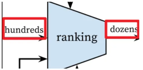
The following figure is the architecture diagram of the recommendation system model of this article. The video pool contains hundreds of millions of videos. When passing through the first layer of the candidate generation layer model, this layer mainly performs rough screening, and the videos are filtered to only hundreds of videos. , when passing through the second layer of the model again, this layer will score and sort the videos, then filter out the top dozens of videos, and output them to the user’s video homepage for users to watch, as shown in the following figure:
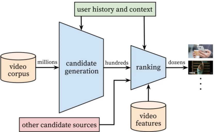
1. CANDIDATE GENERATION candidate generation model
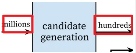
This layer of model can be summed up in two words as “rough”. The tens of billions of videos in the video pool are filtered through the first layer to obtain hundreds of videos, which are then passed to the next layer of model for further training.
The following figure is the model architecture diagram of the candidate generation model. Looking from bottom to top, the browsing history and search history features are embedded into high-level embedded vectors, and other features related to user portraits are also added, such as geographical location, age, gender and other features. , normalize this demographic information to the [0,1] range, splice it with the previous features, and then feed all the features to the upper layer neural network model. After the three-layer neural network, we can see softmax function. Here YouTube regards this problem as a problem of users recommending next watch, which is a multi-classification problem.
Candidate set generation is modeled as a “very large-scale multi-classification” problem, and its classification formula is shown in the following diagram:
At time t, the user accurately classifies the specified video into the first category Uin its specific context .Cwti
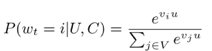
where uis the high-dimensional embedded embedding of the user and its context, vand is the high-dimensional embedded embedding of the video.
Regarding this architecture, the following points deserve attention:
(1) Main feature processing 1: watch and search browsing history and search history.
Videos exist on mobile phones and other devices. They are a series of sparse, variable-length video ID sequences. Through a fixed vocabulary and weighted average, a series of dense, fixed-length viewing vectors can be obtained based on their importance or time. , input into the upper layer neural network, as shown in the figure below:
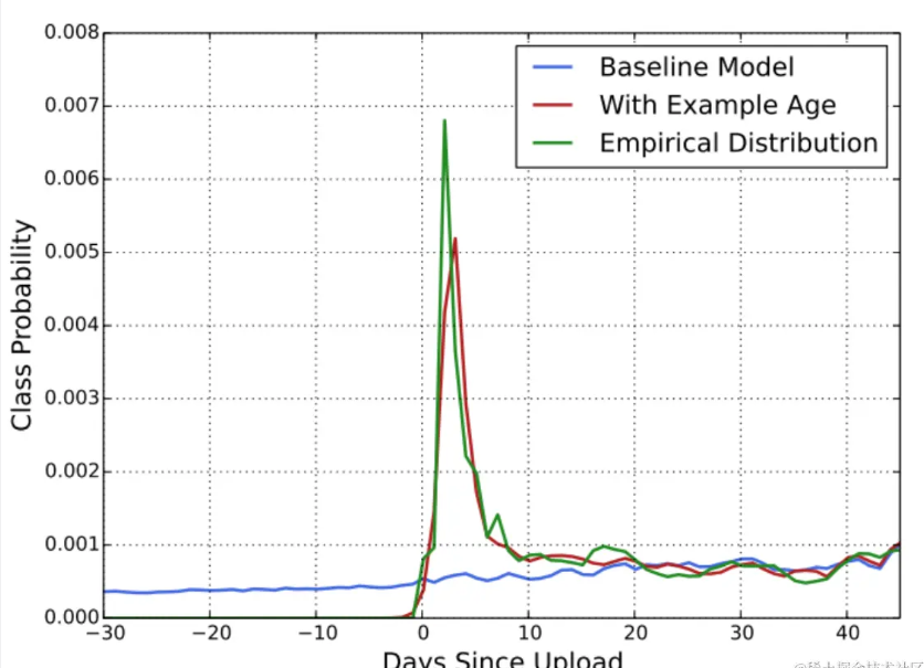
Processing of main features 2: example age video upload time
As shown in the figure below, the abscissa is the time when the video was uploaded, and the axis is the category probability. When the example age feature is not added, you can notice this blue line, which has been performing very mediocrely. After adding this feature, the category The probability is more consistent with the empirical distribution, indicating the importance of this feature.
(2) Context selection
When users watch videos, they follow an asymmetric co-watchasymmetric co-viewing process. When users browse videos, they tend to do so sequentially, starting with some popular videos and gradually finding subdivisions.
As shown in the figure below, (a) uses contextual information to predict the video in the middle, and (b) uses contextual information to predict the video for the next browse. Obviously, predicting the video for the next browse is better than predicting the video in the middle. Video is much simpler.
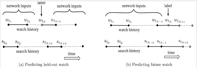
Through experiments, it can also be found that the method in Figure (b) performs better in online A/B test. In fact, traditional collaborative filtering algorithms implicitly use the method in Figure (a), ignoring the asymmetry. Browse mode.
(3) Experiments on feature sets and depth
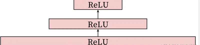
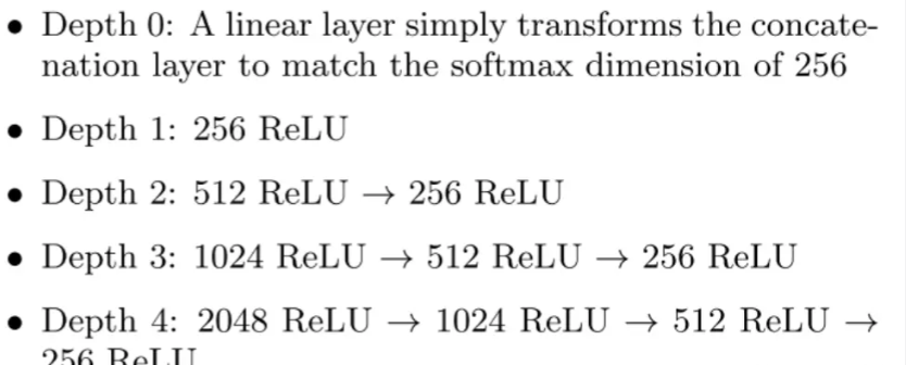
As shown in the figure below, the neural network model uses the classic “tower” mode to build the network. All videos and search histories are embedded into 256-dimensional vectors. The input layer is directly connected to the 256-dimensional softmax layer, and then Increase the network depth in sequence (+512–>+1024–>+2048–>…)
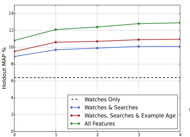
As shown in the figure below, the horizontal axis represents the training depth of the deep neural network, and the vertical axis represents the average accuracy. The independent variable is the number of features. As the number of features increases, the average accuracy shows an upward trend. When the deep neural network reaches the third layer At this time, its average accuracy no longer increases “significantly”.
Of course, taking into account the CPU calculation and the user’s waiting time, the number of layers of the deep neural network should not be too many. Based on experiments, 3 layers of the neural network are enough. Unless future calculations are completed, the training layers of the deep neural network will be infinitely increased. number.
2. RANKING ranking model
The hundreds of models obtained from the previous layer are sorted by the ranking model, and the first dozens of videos are output to the user’s mobile phone for the user to watch.
At first glance, the model architecture of this layer is the same as the first layer candidate generation layer model, but there are some differences. Many other more detailed features have been added for personalized filtering.
Some people will say, why waste all your efforts? Can’t we just build a deep neural network model one by one, score and sort all the videos together, and then output the top dozens of videos to be displayed on the user’s homepage for users to watch? That’s it.
This is indeed possible. How convenient it is to solve it with one model. However, one question you may not have considered is, do current CPUs have such high computing power for your calculations? All users and all videos are sorted and scored separately. Can the server withstand it? Will the CPU calculation be excessive? Even if the calculation can withstand it, how much time will it take? Users who watch videos online cannot afford to wait. There is no doubt that users do not have so much patience and will switch to other software when this recommendation system is finished.
Moreover, it is really unnecessary. For a video that cannot even pass the first level of rough ranking, the score will definitely be too low in the scoring and sorting stage and it will not be ranked at the top.
As shown in the figure above, the ranking model architecture diagram is also viewed from the bottom up. The newly added features include the current video ID to be calculated, the last N IDs that the user has watched, the user’s language, and the language of the video as language embeddings. , as well as features such as the time since the last time the video was watched on the same channel, the number of times the video has been exposed to the user, etc. These features are spliced together and then fed to the upper layer neural network model. During training, weighted logistic regression is used to assign Score independently and sort by score.
For sorting DNN, there are the following points to pay attention to:
(1) The user’s love for the channel can be measured by the number of clicks on the channel’s videos, the user’s last viewing time on the channel, etc.
(2) Category feature embedding: The author generates an independent embedding space for each category feature dimension. It is worth noting that embedding can be shared for features in the same domain, which has the advantage of accelerating iteration and reducing memory overhead.
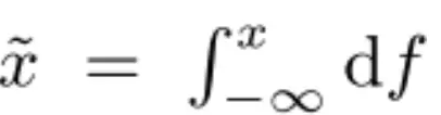
(3) Continuous feature normalization: DNN is sensitive to the distribution of input and the scale of features. The author designs an integral function to map the feature into a variable obeying the [0,1] distribution. The integral function is:
(4) Modeling expected viewing time: Positive sample: the video is shown and clicked; weighted negative sample according to the viewing time: the video is shown but not clicked; unit weight The author uses a weighted logistic regression to train based on cross-entropy loss . The logistic regression odds are:
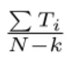
Then the learning probability is: E[T]*(1+P) ≈ E[T] [expected viewing time, click rate]
(5) The fifth feature #previous impressions introduces the idea of exploration to a certain extent to prevent the same video from continuously invalidating the same user. Generally speaking, after a user watches a video, the probability of watching the same video again is greatly reduced, so there is no need to push the video to the user again.
3. Hidden layer experiment
The figure below is an experiment conducted by the author on the number of hidden layers of the neural network model. It can be seen that as the number and width of the hidden layer increase, the weighted loss for each user decreases, reaching 1024–>512- in the experiment. ->256 In this network, the loss is no longer “significantly” reduced, so just choose the hidden layer of this configuration, and the loss is 34.6%.
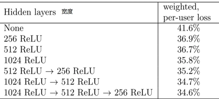
For the network 1024–>512–>256, the loss increased by 0.2% when testing the version that did not include the normalized root and square. And if weighted LR is replaced by LR, the effect drops to 4.1%.
4. CONCLUSIONS Summary
The most prominent contribution of this article is how to combine business reality and user scenarios to select equivalent problems and implement a recommendation system.
First, the deep collaborative filtering model is able to effectively absorb more features and model their interactions with depth layers, outperforming the matrix factorization method previously used on YouTube.
Secondly, the author’s strategy for processing features is full of wisdom. For example, example agethe addition of features removes the inherent bias toward the past and allows the model to represent the time-dependent behavior of popular videos.
Finally, in the sorting stage, the selection of evaluation indicators can be combined with the business, and the expected viewing time can be used for training.
5. Some personal thoughts
This paper is a conference article on recommendation systems published by YouTube in 2016.
YouTube’s recommendation system only uses two models. It uses the deep learning neural network method to make recommendations. Overall, the model is a little simpler, but it is faster. I have used the YouTube software myself and found that its recommendation algorithm does have some shortcomings. Whatever videos you watch, it will always recommend related videos to you. It is too simple. In terms of the recommendation algorithm alone, it is still recommended by some domestic software. good. But after all, it is a recommendation algorithm that has been around for 16 years, and it is the first time that a deep learning neural network has been used in a recommendation system. Moreover, it is a paper that has been implemented in industry. It can be made public for us to read, and it still makes me gain knowledge.